Uniswap V3: Understanding the Real Reserves Curve

Uniswap is currently the leading decentralized exchange in the blockchain world. In this article, I am going to explain the Curve of Real Reserve on Uniswap V3 in mathematical logic. This paper assumes you are familiar with automated market makers between two assets X and Y defined as a trading function, meaning a relationship between its reserves x and y.

First, we consider a market with liquidity L and amounts x and y of assets X and Y respectively. And, we also have P as the price of X in terms of Y.

It follows immediately that:

In the earlier version, Uniswap V2, liquidity was distributed across the entire price range (0,∞), leading to inefficient liquidity utilization since much of the assets in the pool are never touched. The graph looks like this:

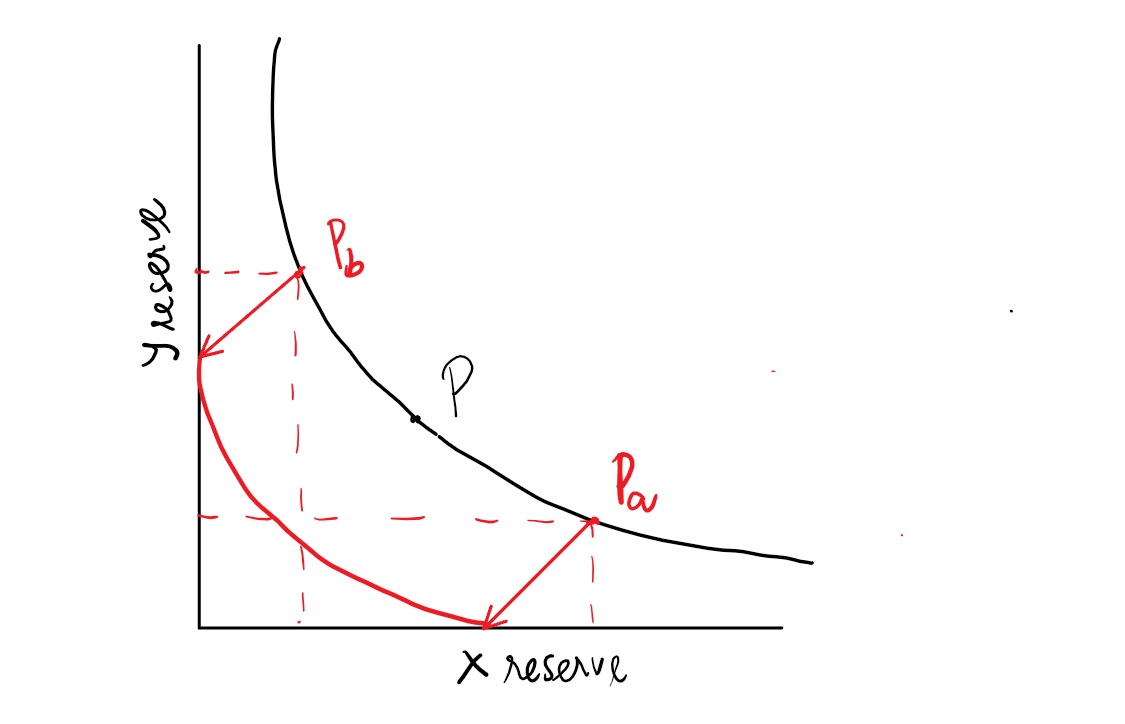
Now, on version V3, liquidity providers are capable of providing liquidity in a fixed price range, saying [Pa, Pb] for example. This feature is called concentrated liquidity. 

If the price does not fall outside of the range, you can provide more effective liquidity called virtual liquidity. Then, we rewrite the reserves x and y in terms of the real and virtual reserves:

With a concentrated position, reserves for both tokens in the pool are consumed at a greater rate during trades, leading them to be fully exhausted at either end of the range (Pa or Pb). 

This means that when P = Pb, the real reserve of token X (x_r) is equal to 0, combine with (3) then we have x_v in terms of L and Pb:

Similarly, when P = Pa, the real reserve of token Y (y_r) is equal to 0:

Lastly, by combining (4) and (5), we can rewrite the version V2 formula in terms of real reserves of two tokens like this: 

This final equation is exactly the mathematical logic representing the Curve of Real Reserves on Uniswap V3.