
Uniswap: How to calculate Impermanent Loss?

Impermanent Loss is a popular concept when it comes to automated market makers and decentralized exchanges like Uniswap. This term is often defined as the percentage loss a liquidity provider would experience for a given price movement. This means that, as an LP, your position may fall in value due to volatility, causing a loss compared to holding these assets outside of the pool. 

This article will spell out the concept in mathematical logic and explain all the assumptions involved. 

We consider a market with liquidity L and amounts x and y of assets X and Y respectively. We also have P as the price of X in terms of Y, and a price movement P1 = P.d where d >0

According to the definition of IL touched upon, we establish a generic formula for IL:

where:
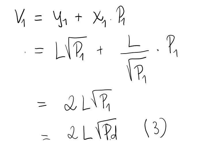
  • V1 is the value of your position in the pool at the price P1 (x,y move with price)
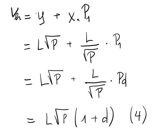
  • Vh is the value of your assets at the price P1 if you keep them outside of the pool 
  • We also consider V0 as the initial value of your holding (at the price P)

Impermanent Loss on Uniswap V2

On Uniswap V2, we have constant product formula and the price between X and Y:


It follows then that:


When the price move to P1, we have V1 in terms of L and P1:

and also have Vh in terms of L and P1:


By combining (3) and (4), we can easily derive the formula for IL:


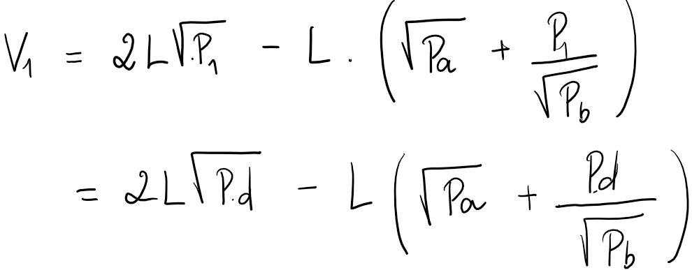
Impermanent Loss on Uniswap V3

On the Uniswap V3, reserves for a concentrated position are described by the curve:


We will use the same approach to calculate IL for V3 based on the above V2 section, and also define Pa, Pb to be the price interval for our concentrated position. Both P and P1 are assumed to be inside this range. 

On the other hand, we can also determine the amounts x and y in terms of real and virtual reserves. And note that the amounts of reserves of your position are now x_r and y_r:

Now, we combine (1), (2) with the V3 curve, then the real reserves are described like this:


The initial value V0 of your holding:


When the price move to P1, the real reserves x_r and y_r also change and V1 is just V0 with P1 substituted for P:

Next up is Vh:

Finally, we calculate IL on V3 as a percentage change:

We also can described IL(V3) in terms of IL(V2): 


Note that we don't use this equation if the price falls outside the liquidity range [Pa, Pb].


Comments

Popular posts from this blog

DeFi Summary Q3 2022

DeFi protocols have begun to shift in their business life cycle, with some dApps even showing periods of profitability  Regulatory Actions Q3 has been an active period for regulators. The US SEC claimed that it has jurisdiction over Ethereum transactions because nodes are clustered more densely in the US than in any other country. According to Ehernode's data, roughly 45% of Ethereum validator nodes operate from the US, with Germany in a distant second at 12% and Singapore at 4%. Below it shows the estimated geographic distribution of Ethereum nodes worldwide.  In August, the US Treasury sanctioned the cryptocurrency mixer, Tornado Cash. This is seemingly the first time the Treasury sanctioned a piece of code (as opposed to an individual or entity) but likely not the last. The CFTC has also been active, issuing a settlement order finding that Ooki DAO and its founders violated the Commodity Exchange Act and applying a $250k fine. The Commission defines the Ooki DAO unincorpora...

Uniswap V3: Understanding the Real Reserves Curve

Uniswap is currently the leading decentralized exchange in the blockchain world. In this article, I am going to explain the Curve of Real Reserve on Uniswap V3 in mathematical logic. This paper assumes you are familiar with automated market makers between two assets X and Y defined as a trading function, meaning a relationship between its reserves x and y. First, we consider a market with liquidity L and amounts x and y of assets X and Y respectively. And, we also have P as the price of X in terms of Y. It follows immediately that: In the earlier version, Uniswap V2, liquidity was distributed across the entire price range (0,∞), leading to inefficient liquidity utilization since much of the assets in the pool are never touched. The graph looks like this: Now, on version V3, liquidity providers are capable of providing liquidity in a fixed price range, saying [Pa, Pb] for example. This feature is called concentrated liquidity.  If the price does not fall outside of the range, you ca...